Symmetric Chaos with Datashader and Numba

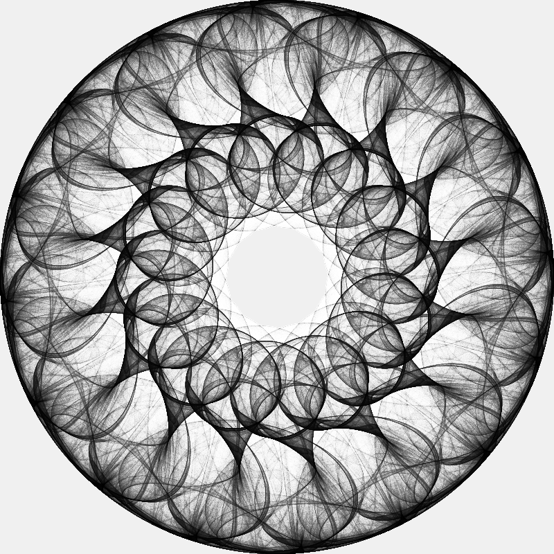
Map equation and coefficient values are taken from here. Some mathematical explainations can be found here, by Mike Field and Martin Golubitsky.

import numpy as np
import pandas as pd
import datashader as ds
from datashader import transfer_functions as tf
import numba
from numba import jit
import matplotlib
import matplotlib.pyplot as plt
import warnings
warnings.filterwarnings("ignore")
import sys

print(f"Python version: {sys.version}")
print(f"Numpy version: {np.__version__}")
print(f"Pandas version: {pd.__version__}")
print(f"Datashader version: {ds.__version__}")
print(f"Matplotlib version: {matplotlib.__version__}")

Python version: 3.7.0 (default, Jun 28 2018, 13:15:42) 
[GCC 7.2.0]
Numpy version: 1.15.1
Pandas version: 0.23.4
Datashader version: 0.6.6
Matplotlib version: 2.2.3

# image size
width = 800
height = 800
cvs = ds.Canvas(plot_width=width, plot_height=height)

# number of steps
n = 100000000

# colormap
greys = plt.get_cmap('Greys')
bckgrnd = (240, 240, 240)

@jit
def map(x, y, alph, bet, gamm, omeg, lambd, deg):
    zzbar = x * x + y * y
    p = alph * zzbar + lambd
    zreal, zimag = x, y
    for i in range(1, deg-1):
        za, zb = zreal * x - zimag * y, zimag * x + zreal * y
        zreal, zimag = za, zb
    zn = x * zreal - y * zimag
    p += bet * zn
    return p * x + gamm * zreal - omeg * y, \
           p * y - gamm * zimag + omeg * x

@jit
def trajectory(alph, bet, gamm, omeg, lambd, deg, x0=0.01, y0=0.01, n=n):
    x, y = np.zeros(n), np.zeros(n)
    x[0], y[0] = x0, y0
    for i in np.arange(n-1):
        x[i+1], y[i+1] = map(x[i], y[i], alph, bet, gamm, omeg, lambd, deg)
    return pd.DataFrame(dict(x=x,y=y))

def compute_and_plot(alph, bet, gamm, omeg, lambd, deg, n=n):
    df = trajectory(alph, bet, gamm, omeg, lambd, deg)[1000:]
    agg = cvs.points(df, 'x', 'y')
    img = tf.shade(agg, cmap=greys)
    img = tf.set_background(img, bckgrnd)
    return img

%%time
compute_and_plot(1.8, 0.0, 1.0, 0.1, -1.93, 5)

CPU times: user 4.61 s, sys: 1.22 s, total: 5.84 s
Wall time: 4.45 s

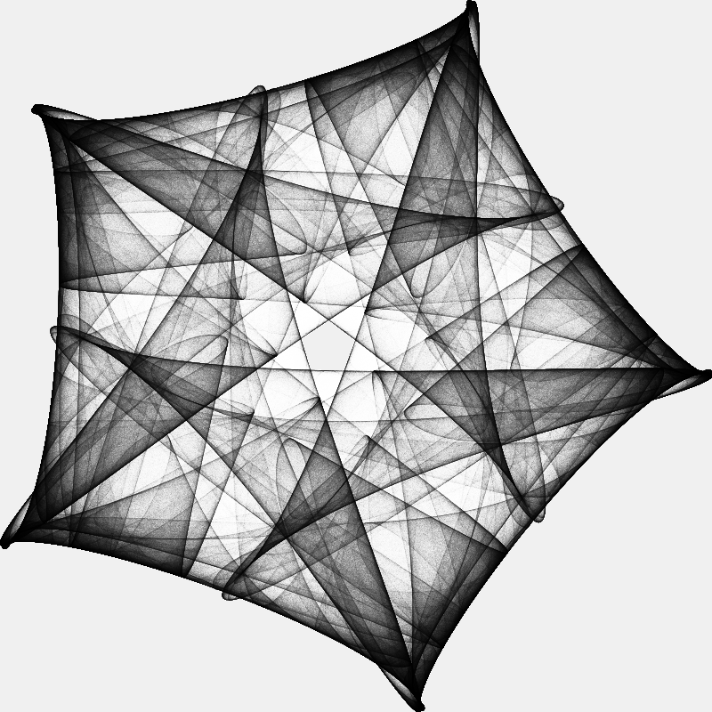
%%time
compute_and_plot(5.0, -1.0, 1.0, 0.188, -2.5, 5)

CPU times: user 4.15 s, sys: 1.28 s, total: 5.43 s
Wall time: 3.79 s

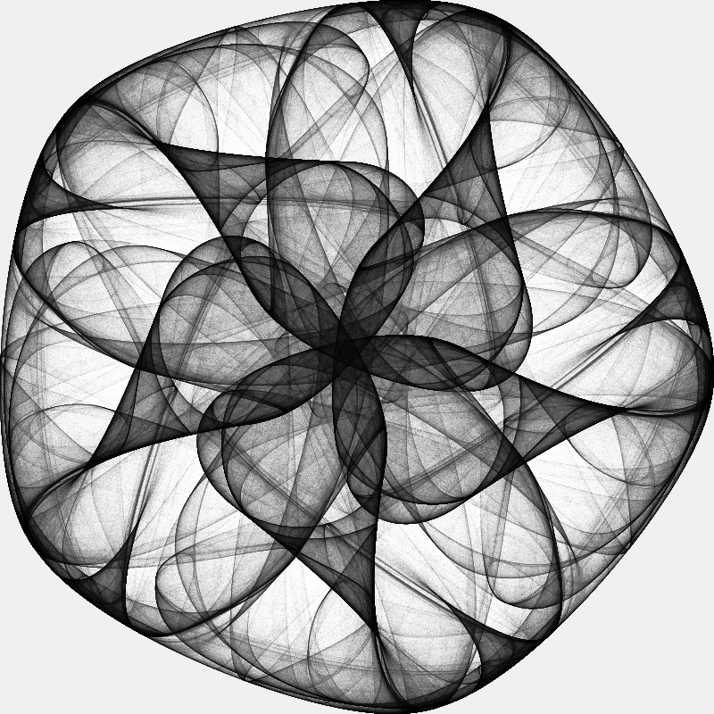
%%time
compute_and_plot(-1.0, 0.1, -0.82, 0.12, 1.56, 3)

CPU times: user 3.77 s, sys: 1.41 s, total: 5.18 s
Wall time: 3.37 s

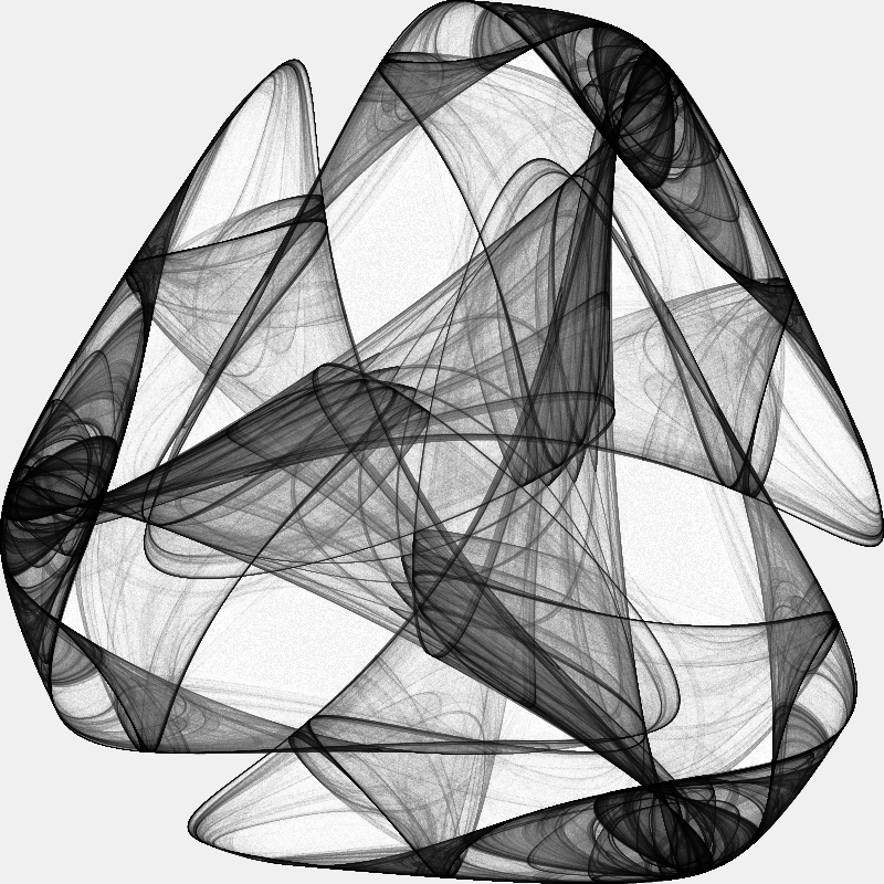
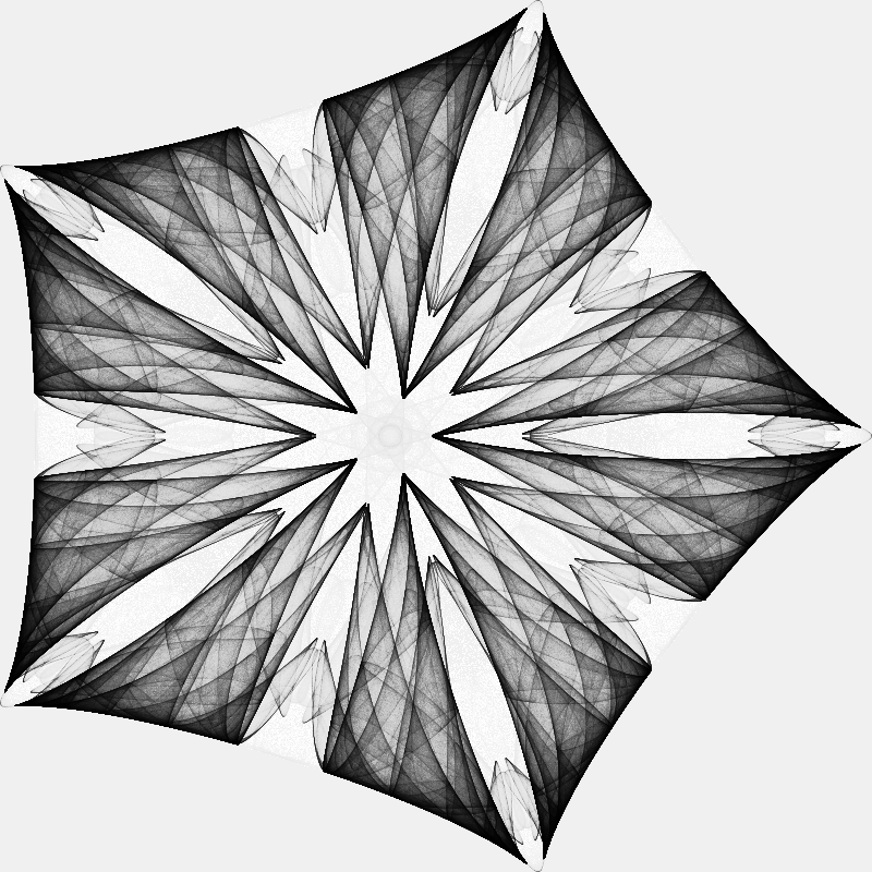
%%time
compute_and_plot(1.806, 0.0, 1.0, 0.0, -1.806, 5)

CPU times: user 4.13 s, sys: 1.28 s, total: 5.41 s
Wall time: 3.75 s

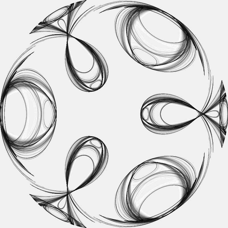
%%time
compute_and_plot(10.0, -12.0, 1.0, 0.0, -2.195, 3)

CPU times: user 3.7 s, sys: 1.41 s, total: 5.11 s
Wall time: 3.29 s

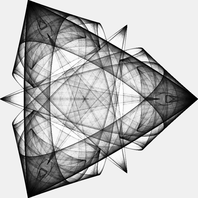
%%time
compute_and_plot(-2.5, 0.0, 0.9, 0.0, 2.5, 3)

CPU times: user 3.48 s, sys: 1.24 s, total: 4.72 s
Wall time: 3.2 s

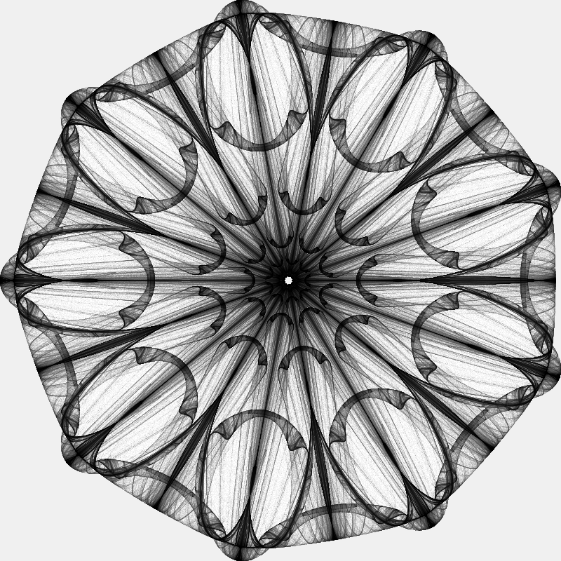
%%time
compute_and_plot(3.0, -16.79, 1.0, 0.0, -2.05, 9)

CPU times: user 5.23 s, sys: 1.18 s, total: 6.4 s
Wall time: 4.81 s

%%time
compute_and_plot(5.0, 1.5, 1.0, 0.0, -2.7, 6)

CPU times: user 4.35 s, sys: 1.45 s, total: 5.8 s
Wall time: 4.06 s

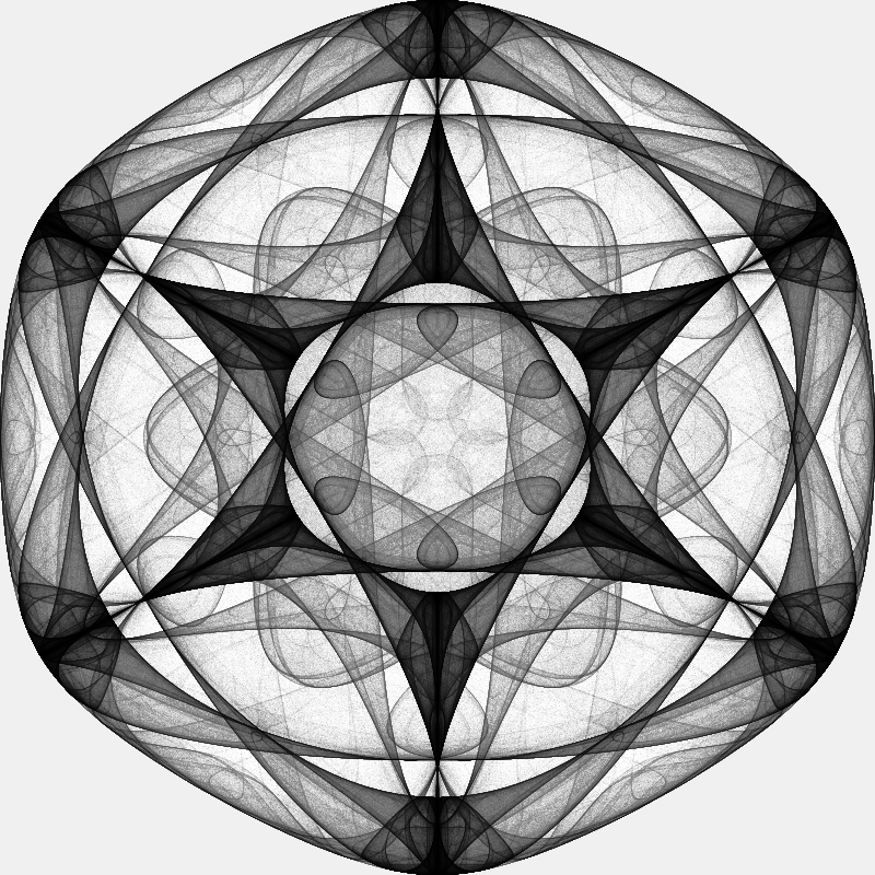
%%time
compute_and_plot(-2.5, 0.0, 0.9, 0.0, 2.409, 23)

CPU times: user 8.97 s, sys: 1.23 s, total: 10.2 s
Wall time: 8.64 s

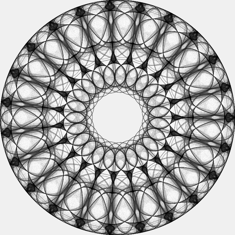
%%time
compute_and_plot(1.0, -0.1, 0.167, 0.0, -2.08, 7)

CPU times: user 4.74 s, sys: 1.29 s, total: 6.04 s
Wall time: 4.3 s

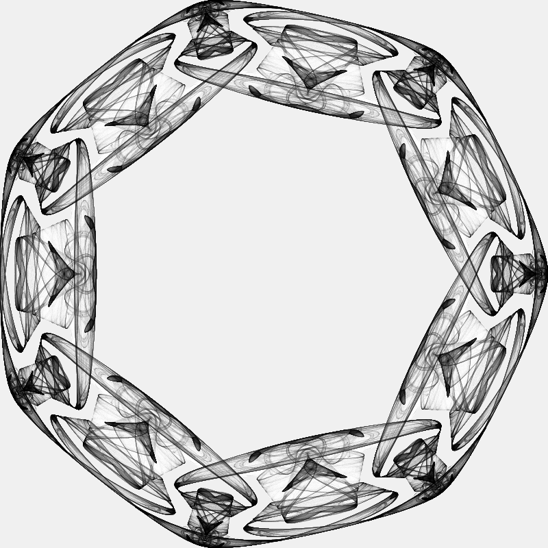
%%time
compute_and_plot(2.32, 0.0, 0.75, 0.0, -2.32, 5)

CPU times: user 4.02 s, sys: 1.25 s, total: 5.27 s
Wall time: 3.72 s

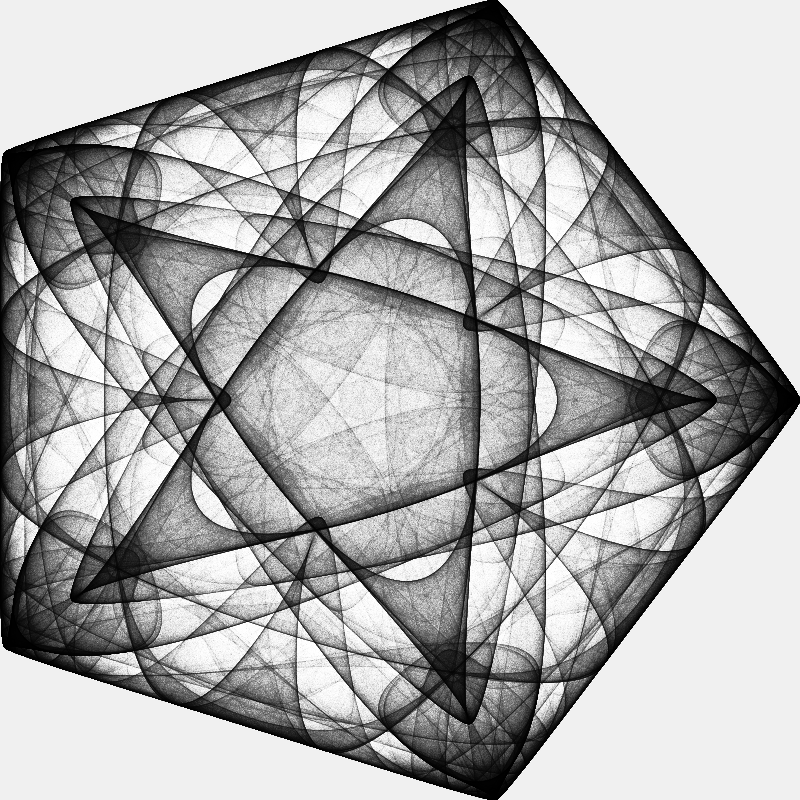
%%time
compute_and_plot(-2.0, 0.0, -0.5, 0.0, 2.6, 5)

CPU times: user 4.04 s, sys: 1.29 s, total: 5.33 s
Wall time: 3.74 s

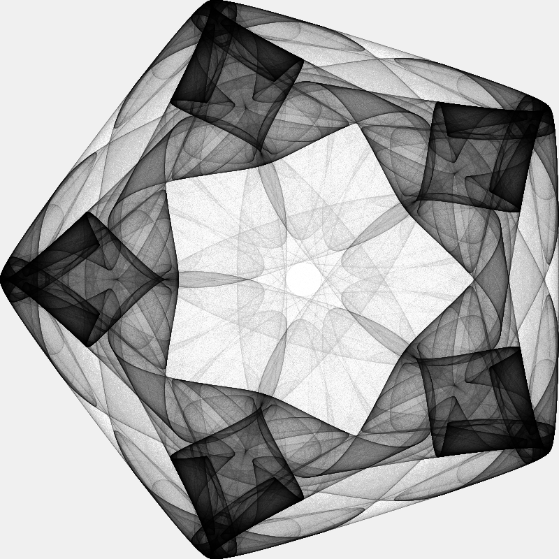
%%time
compute_and_plot(2.0, 0.2, 0.1, 0.0, -2.34, 5)

CPU times: user 4.06 s, sys: 1.27 s, total: 5.32 s
Wall time: 3.71 s

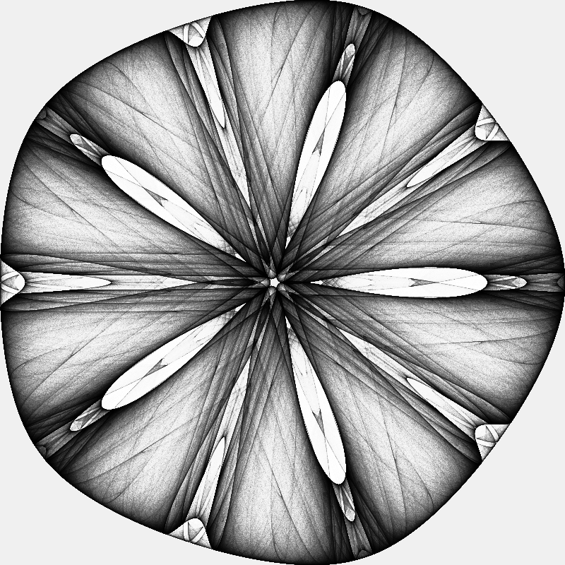
%%time
compute_and_plot(2.0, 0.0, 1.0, 0.1, -1.86, 4)

CPU times: user 3.87 s, sys: 1.54 s, total: 5.41 s
Wall time: 3.59 s

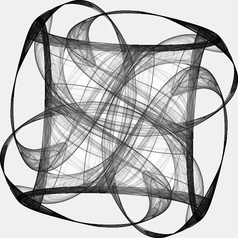
%%time
compute_and_plot(-1.0, 0.1, -0.82, 0.0, 1.56, 3)

CPU times: user 3.68 s, sys: 1.35 s, total: 5.03 s
Wall time: 3.29 s

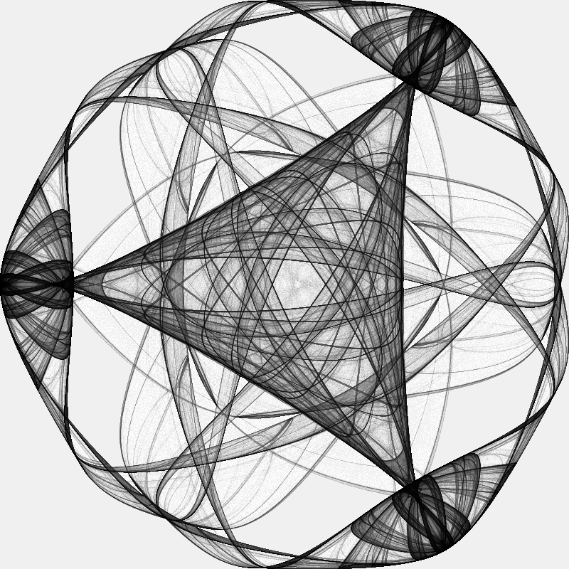
%%time
compute_and_plot(-1.0, 0.1, -0.805, 0.0, 1.5, 3)

CPU times: user 3.59 s, sys: 1.23 s, total: 4.83 s
Wall time: 3.26 s

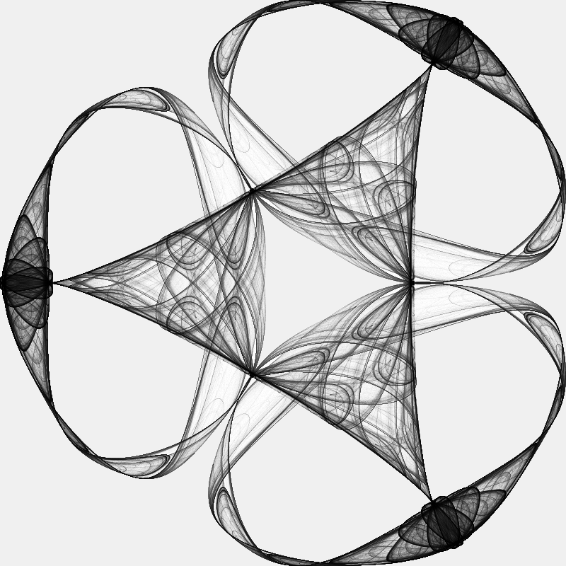
%%time
compute_and_plot(-1.0, 0.03, -0.8, 0.0, 1.455, 3)

CPU times: user 3.54 s, sys: 1.35 s, total: 4.89 s
Wall time: 3.18 s

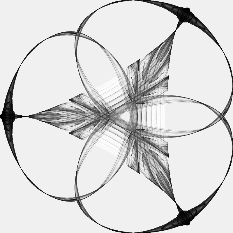
%%time
compute_and_plot(-2.5, -0.1, 0.9, -0.15, 2.39, 16)

CPU times: user 6.99 s, sys: 1.28 s, total: 8.28 s
Wall time: 6.73 s