In this short post, we are using the Global Human Settlement Layer from the European Commission:

This spatial raster dataset depicts the distribution of population, expressed as the number of people per cell.

The downloaded file has a worldwide resolution of 250m, with a World Mollweide coordinates reference system. Values are expressed as decimals (float32) and represent the absolute number of inhabitants of the cell. A value of -200 is found whenever there is no data (e.g. in the oceans). Also, it corresponds to the 2015 population estimates.

We are going to load the data into a xarray DataArray and make some plots with Datashader.

Datashader is a graphics pipeline system for creating meaningful representations of large datasets quickly and flexibly.

Imports

import rioxarray
import xarray as xr
import datashader as ds
from datashader import transfer_functions as tf
from colorcet import palette

FP = "GHS_POP_E2015_GLOBE_R2019A_54009_250_V1_0.tif"  # file path

Loading the dataset

Let's start by opening the file using rioxarray, and dask as backend. rioxarray is a geospatial xarray extension powered by rasterio.

da = rioxarray.open_rasterio(
    FP,
    chunks=True,
    lock=False,
)

type(da)

xarray.core.dataarray.DataArray

Total population

Let's compute the total population count:

%%time
total_pop = da.where(da[0] > 0).sum().compute()
total_pop = float(total_pop.values)

CPU times: user 4min 45s, sys: 22.5 s, total: 5min 8s
Wall time: 40.8 s

print(f"Total population : {total_pop}")

Total population : 7349329920.0

World population was indeed around 7.35 billion in 2015.

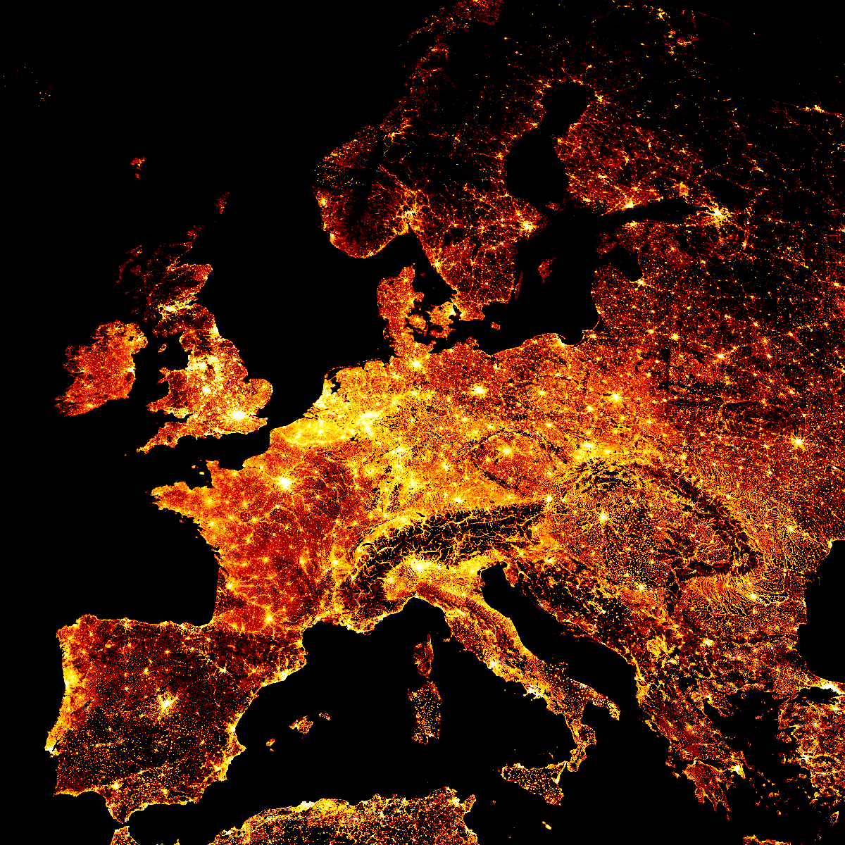
Europe

Let's focus on Europe with a bounding box in World_Mollweide coordinates:

minx = float(da.x.min().values)
maxx = float(da.x.max().values)
miny = float(da.y.min().values)
maxy = float(da.y.max().values)
print(f"minx : {minx}, maxx : {maxx}, miny : {miny}, maxy : {maxy}")

minx : -18040875.0, maxx : 18040875.0, miny : -8999875.0, maxy : 8999875.0

So let's clip the data array using a bounding box:

dac = da.rio.clip_box(
    minx=-1_000_000.0,
    miny=4_250_000.0,
    maxx=2_500_000.0,
    maxy=7_750_000.0,
)

And plot this selection:

dac0 = xr.DataArray(dac)[0]
dac0 = dac0.where(dac0 > 0)
dac0 = dac0.fillna(0.0).compute()

size = 1200
cvs = ds.Canvas(plot_width=size, plot_height=size)
raster = cvs.raster(dac0)

We are using the default mean downsampling operation to produce the image.

cmap = palette["fire"]
img = tf.shade(
    raster, how="eq_hist", cmap=cmap
)
img

France

We are now going to focus on France, by cliping /re-projecting/re-cliping the data:

dac = da.rio.clip_box(
    minx=-450_000.0,
    miny=5_000_000.0,
    maxx=600_000.0,
    maxy=6_000_000.0,
)

dacr = dac.rio.reproject("EPSG:2154")

minx = float(dacr.x.min().values)
maxx = float(dacr.x.max().values)
miny = float(dacr.y.min().values)
maxy = float(dacr.y.max().values)
print(f"minx : {minx}, maxx : {maxx}, miny : {miny}, maxy : {maxy}")

minx : 3238.8963631442175, maxx : 1051199.0429940927, miny : 6088320.296559229, maxy : 7160193.962105454

dacrc = dacr.rio.clip_box(
    minx=80_000,
    miny=6_150_000,
    maxx=1_100_000,
    maxy=7_100_000,
)

dac0 = xr.DataArray(dacrc)[0]
dac0 = dac0.where(dac0 > 0)
dac0 = dac0.fillna(0.0).compute()

cvs = ds.Canvas(plot_width=size, plot_height=size)
raster = cvs.raster(dac0)

cmap = palette["fire"]
img = tf.shade(raster, how="eq_hist", cmap=cmap)
img

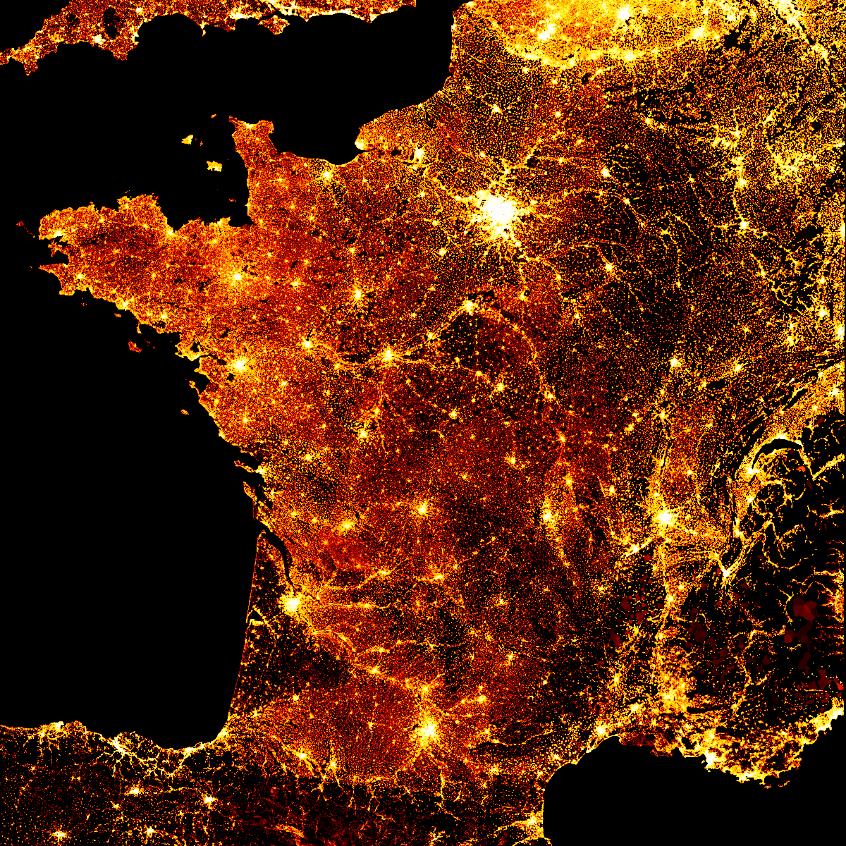
We can notice that some areas are not detailed up to the 250m accuracy, but rather averaged over larger regions, exhibiting a uniform color (e.g. in the southern Alps).