

In this blog post, we will show how to use Python to simulate the amortization of a fully amortized loan, such as a mortgage or a car loan. We will derive the formula for calculating the monthly payments and the outstanding balance, and implement them in Python using Numba. We will also use the IPyWidgets library to create interactive widgets that will allow us to explore the effects of different loan parameters on the amortization schedule.
Amortization formulas
When you take out a loan, you typically agree to repay the loan in equal monthly installments over a fixed period of time. This type of loan is known as a fully amortized loan. We will use the following variables in our derivation:
: the principal amount borrowed
: the total number of monthly payments
: the annual interest rate
: the monthy interest rate
: the principal part of monthly payment
: the interest part of monthly payment
: the constant monthly payment
: the balance [principal still due] after the -th payment
We have the following identities:
Since , and are known, it is easy to compute . However, we need to compute eather or in order to be able to perform the simulation. Here is the derivation of the formula.
It is easy to show by recursion that:
Indeed, we have , and:
By summing up all the terms, we get:
And so:
For , the denominator of the fraction can be simplified in the following way:
This leads to:
And eventually:
Imports
In the next section, we will implement these formulas in Python. First, let's import the necessary libraries:
import ipywidgets as widgets
import numpy as np
import pandas as pd
from ipywidgets import interact
from numba import jit
We are operating on Python version 3.11.5 and running on a Linux x86_64 machine.
ipywidgets             : 8.0.7
numpy                  : 1.24.4
pandas                 : 2.1.3
numba                  : 0.57.1
Implementing the Amortization Formulas in Python
@jit(nopython=True)
def _compute_amortized_loan_inner(a, r, mc):
    """
    a: amount, r: annual interest rate, mc: month count
    """
    P = np.empty(mc, dtype=np.float64)  # principal part
    I = np.empty(mc, dtype=np.float64)  # interest part
    B = np.empty(mc, dtype=np.float64)  # balance

    # init
    if r > 0.0:
        P[0] = r * a / (12.0 * ((1.0 + r / 12.0) ** mc - 1.0))
    else:
        P[0] = a / mc
    I[0] = r * a / 12.0
    t = I[0] + P[0]
    B[0] = a - P[0]

    # loop on months
    for m in range(1, mc):
        I[m] = r * B[m - 1] / 12.0
        P[m] = t - I[m]
        B[m] = B[m - 1] - P[m]

    return P, I, B, t


def compute_amortized_loan(amount=200_000, interest_rate_pc=4.0, period_m=180):
    """Compute the amortization schedule for a fully amortized loan.

    Parameters
    ----------
    amount : float
        The principal amount borrowed.
    interest_rate_pc : float
        The annual interest rate, in percentage points.
    period_m : int
        The total number of monthly payments.

    Returns
    -------
    df : pandas.DataFrame
        A DataFrame containing the amortization schedule, with one row for
        each monthly payment. The columns of the DataFrame are:

        * `principal`: the principal part of the monthly payment
        * `interest`: the interest part of the monthly payment
        * `balance`: the outstanding balance after the monthly payment
        * `total`: the total monthly payment
    """

    r = 0.01 * interest_rate_pc

    P, I, B, t = _compute_amortized_loan_inner(amount, r, period_m)

    df = pd.DataFrame(
        data={"principal": P, "interest": I, "balance": B},
        index=np.arange(1, period_m + 1),
    )
    df.rename_axis("month", inplace=True)
    df["total"] = t

    return df
Now we can use the compute_amortized_loan function to calculate the amortization schedule for a loan of $200,000 with an annual interest rate of 3.5% over a period of 180 months (15 years).
%%time
df = compute_amortized_loan(amount=200_000, interest_rate_pc=3.5, period_m=180)
CPU times: user 709 ms, sys: 1.31 s, total: 2.02 s
Wall time: 316 msdf.head(3)| principal | interest | balance | total | |
|---|---|---|---|---|
| month | ||||
| 1 | 846.431749 | 583.333333 | 199153.568251 | 1429.765083 |
| 2 | 848.900509 | 580.864574 | 198304.667742 | 1429.765083 |
| 3 | 851.376468 | 578.388614 | 197453.291274 | 1429.765083 |
df.tail(3)| principal | interest | balance | total | |
|---|---|---|---|---|
| month | ||||
| 178 | 1417.327263 | 12.437820 | 2.847068e+03 | 1429.765083 |
| 179 | 1421.461134 | 8.303949 | 1.425607e+03 | 1429.765083 |
| 180 | 1425.607062 | 4.158021 | -5.029506e-10 | 1429.765083 |
One aspect not addressed in this simulation is the rounding of results to two decimal places, which could be a consideration for future refinements.
Plot
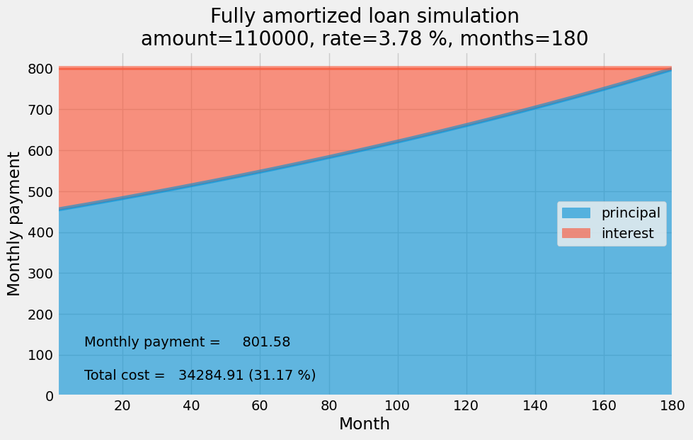
We will now create static and interactive visualizations of the amortization schedule.
Static
def plot_amortized_loan(amount=100_000, interest_rate_pc=3.5, period_m=180):
    df = compute_amortized_loan(amount, interest_rate_pc, period_m)
    ax = df[["principal", "interest"]].plot.area(
        stacked=True, alpha=0.6, figsize=(10, 6)
    )
    cost = (df.total - df.principal).sum()
    total = df.total.values[0]
    ax.legend(loc="center right")
    _ = ax.set_xlim(1, period_m)
    _ = plt.text(
        x=0.05 * period_m, y=0.15 * total, s=f"Monthly payment = {total:10.2f}"
    )
    _ = plt.text(
        x=0.05 * period_m,
        y=0.05 * total,
        s=f"Total cost = {cost:10.2f} ({100.*cost/amount:.2f} %)",
    )
    _ = ax.set(
        title=f"Fully amortized loan simulation\namount={amount:.0f}, rate={interest_rate_pc:.2f} %, months={period_m}",
        xlabel="Month",
        ylabel="Monthly payment",
)plot_amortized_loan(amount=110_000, interest_rate_pc=3.78, period_m=180)
Interactive
We will now use the IPyWidgets library to create interactive widgets that will allow us to explore the effects of different loan parameters on the amortization schedule.
_ = interact(
    plot_amortized_loan,
    amount=widgets.FloatSlider(
        value=200000,
        min=10000,
        max=250000,
        step=1000,
        description="Amount",
        continuous_update=False,
        readout_format=".0f",
    ),
    interest_rate_pc=widgets.FloatSlider(
        value=3.5,
        min=0.0,
        max=7.5,
        step=0.01,
        description="Rate (%)",
        continuous_update=False,
        readout_format=".2f",
    ),
    period_m=widgets.IntSlider(
        value=120,
        min=2,
        max=360,
        step=1,
        description="Months",
        continuous_update=False,
        readout_format="d",
    ),
)
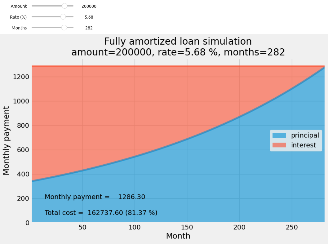
Thanks to Numba, each adjustment made using a slider widget triggers a swift response, leading to an almost instantaneous update of the figure in the Jupyter notebook.
References
[1] Bret D. Whissel, A Derivation of Amortization, https://www.bretwhissel.net/amortization/amortize2col.pdf


